SedimentLoadAnalysis
1. Sediment Concentration ((C)):
Sediment concentration is a measure of the amount of sediment present in water, typically expressed in terms of mass per unit volume. It is commonly denoted in units of milligrams per liter (mg/L) or parts per million (ppm). The sediment concentration ((C)) can be calculated using the formula:
C = m/v
where:
- ( C ) is the sediment concentration (mg/L or ppm),
- ( m ) is the mass of sediment (in milligrams),
- ( V ) is the volume of water (in liters).
2. Sediment Load ((SSL)):
Sediment load represents the total quantity of sediment transported by a river or stream over a specific period. It is the product of sediment concentration ((C)) and discharge ((Q)) and is typically expressed in mass units. The formula for sediment load is:
[ SSL = C x Q ]
where:
- ( SSL ) is the sediment load (in kilograms or metric tons),
- ( C ) is the sediment concentration (mg/L or kg/m³),
- ( Q ) is the discharge or flow rate of water (in cubic meters per second).
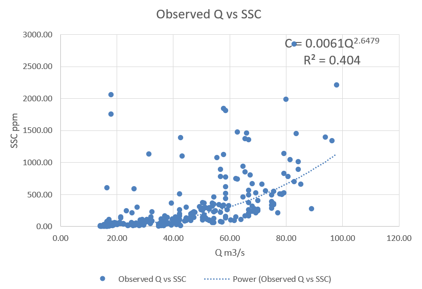
3. Curve of Discharge vs. Suspended Sediment Concentration (Q vs. SSC):
The curve of discharge vs. suspended sediment concentration represents the relationship between the flow rate (discharge) of a river or stream and the concentration of suspended sediment in the water. This curve is often referred to as the sediment rating curve or sediment-discharge curve. It provides insights into how sediment concentration varies with changes in flow.
The formula for the sediment rating curve can take the form of a power-law relationship, often expressed as:
[ C = aQ^b ]
where:
- ( C ) is the sediment concentration (mg/L or kg/m³),
- ( Q ) is the discharge (cubic meters per second),
- ( a ) and ( b ) are coefficients to be determined through regression analysis.
The curve is obtained by plotting observed data points of discharge vs. sediment concentration and fitting a regression model to the data to determine the values of ( a ) and ( b ).
These concepts are fundamental in sediment transport studies, where understanding the relationship between water flow and sediment transport is crucial for managing water resources and assessing environmental impacts.
Certainly! Let’s create a detailed tutorial for the given scenario. We’ll cover the steps for calculating sediment load, establishing a relationship between discharge ((Q)) and sediment concentration ((C)), and using the Solver method for bias correction.
Step 1: Determine Discharge ((Q)) Using the Rating Curve
 1.1 Rating Curve Equations:
- Use the provided rating curve equations to determine discharge ((Q)) based on gauge height ((h)).
Using Equation of rating curve we can find discharge,
Lets take equations
Q = 3.7(H- 551.3)^2.78 for h < 3m
and Q = 12.22(H- 551.3)^2.0 for h>= 3m
where ( H = h + 552.6 ) masl.
Step 2: Calculate Average Discharge Q_avg and Average Concentration SSC_avg
2.1 Average Discharge and Concentration:
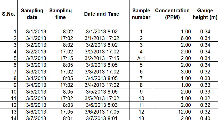
- For each sampling period, calculate the discharge using the rating curve.
- Average the discharge values for a given time period to get Q_avg.
- Calculate the average concentration SSC_avg based on recorded concentration values.
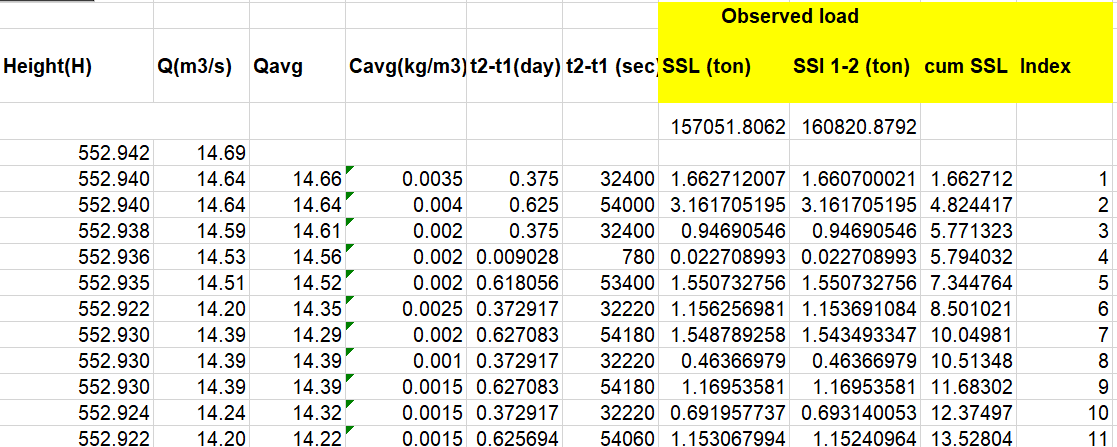
2.2 Sediment Load using two methods
- now we can find SSL ( two methods are used) SSL observed…
- SSL = Qavg x Cavg(kg/m3) x time interval in seconds / 1000 –> ton
- SSL 1-2 = 0.5x(Q1xC1 + Q2xC2)xtime interval in seconds / 1000 —> ton
Step 3: Establish the Relationship between (Q) and (C)
3.1 Curve Fitting:
- Plot (Q) vs (C) using the available data.
- Fit a power-law equation to the data: (C = a*Q^b).
- Determine the values of (a) and (b).
Step 4: Calculate Sediment Load Using Best Fit Equation
4.1 Calculate SSL from Best Fit:
- Use the best-fit equation to calculate (C) based on observed (Q) values.
- Determine sediment load using the formula:
(SSL_predicted = Q_observed * C_predicted * {time interval in seconds} / 1000).
Step 5: Use Solver for Bias Correction
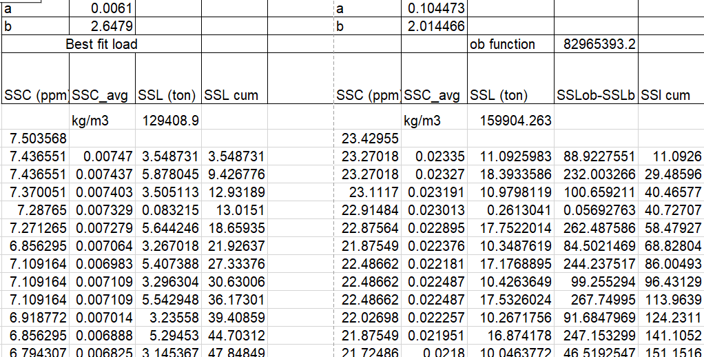
5.1 Objective Function:
Formulate an objective function to minimize the sum of squared differences between observed and predicted sediment loads:
Z = sum [(SSL_observed - SSL_predicted)^2 ]
5.2 Solver Setup:
- Set up Solver in Excel to minimize the objective cell by adjusting the parameters ((a) and (b)).
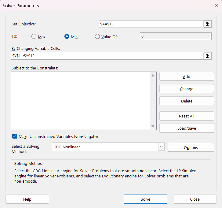
5.3 Run Solver:
- Run Solver to find the parameter values that minimize the objective function.5.4 Evaluate Results:
- Check the final parameter values and the minimized value of the objective function.
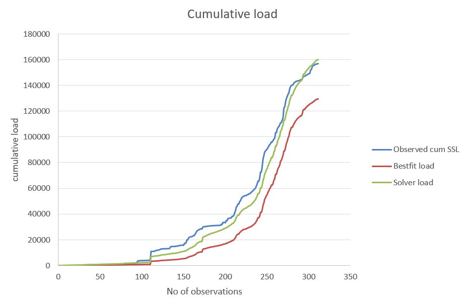
Step 6: Visualize Results
6.1 Plotting:
- Plot results from diffrent process and interpret.